Discretizing the 2D Heat Equation with Radiative Boundary Conditions

The transient temperature field is governed by
\[ \rho c \frac{\partial T}{\partial t} = k\left( \frac{\partial^2 T}{\partial x^2} + \frac{\partial^2 T}{\partial y^2} \right) + Q(x,y,t), \]
where \(T(x,y,t)\) is the temperature field, \(\rho\) is the density, \(c\) is the specific heat, \(k\) is the thermal conductivity, and \(Q(x,y,t)\) is the applied heat source.

The rectangular domain is discretized on a uniform Cartesian grid,
\[ x_i = i\Delta x, \qquad y_j = j\Delta y, \qquad t^n = n\Delta t, \]
with nodal temperatures defined by
\[ T_{i,j}^n \approx T(x_i,y_j,t^n). \]

Using forward Euler in time and second-order central differences in space gives
\[ \frac{\partial T}{\partial t}\Big|_{i,j}^n \approx \frac{T_{i,j}^{n+1}-T_{i,j}^n}{\Delta t}, \]
\[ \frac{\partial^2 T}{\partial x^2}\Big|_{i,j}^n \approx \frac{T_{i+1,j}^n-2T_{i,j}^n+T_{i-1,j}^n}{\Delta x^2}, \]
\[ \frac{\partial^2 T}{\partial y^2}\Big|_{i,j}^n \approx \frac{T_{i,j+1}^n-2T_{i,j}^n+T_{i,j-1}^n}{\Delta y^2}. \]

Substituting these approximations into the PDE yields the explicit interior-node update
\[ T_{i,j}^{n+1} = T_{i,j}^n + \frac{\Delta t}{\rho c} \left[ k\left( \frac{T_{i+1,j}^n-2T_{i,j}^n+T_{i-1,j}^n}{\Delta x^2} + \frac{T_{i,j+1}^n-2T_{i,j}^n+T_{i,j-1}^n}{\Delta y^2} \right) + Q_{i,j}^n \right]. \]

It is convenient to define the diffusion numbers
\[ r_x = \frac{k\Delta t}{\rho c\,\Delta x^2}, \qquad r_y = \frac{k\Delta t}{\rho c\,\Delta y^2}, \]
so that the update becomes
\[ T_{i,j}^{n+1} = T_{i,j}^n + r_x\left(T_{i+1,j}^n-2T_{i,j}^n+T_{i-1,j}^n\right) + r_y\left(T_{i,j+1}^n-2T_{i,j}^n+T_{i,j-1}^n\right) + \frac{\Delta t}{\rho c}Q_{i,j}^n. \]

Heat loss on the left, right, and top boundaries is modeled with a nonlinear radiative boundary condition,
\[ k\frac{\partial T}{\partial n} = -\sigma\epsilon\left(T^4-T_\infty^4\right). \]

Using a one-sided difference at a boundary node gives the nonlinear residual
\[ f(T_b) = k\frac{T_b-T_{\mathrm{in}}}{\Delta} + \sigma\epsilon\left(T_b^4-T_\infty^4\right) = 0, \]
with derivative
\[ f'(T_b) = \frac{k}{\Delta} + 4\sigma\epsilon T_b^3. \]

The boundary temperature is therefore updated iteratively at each time step using Newton--Raphson,
\[ T_b^{(m+1)} = T_b^{(m)} - \frac{f\!\left(T_b^{(m)}\right)}{f'\!\left(T_b^{(m)}\right)}. \]

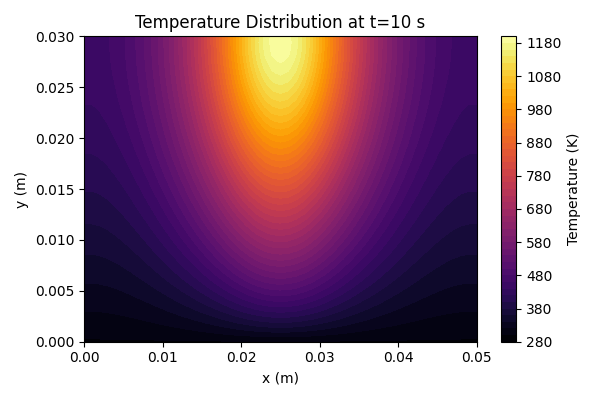
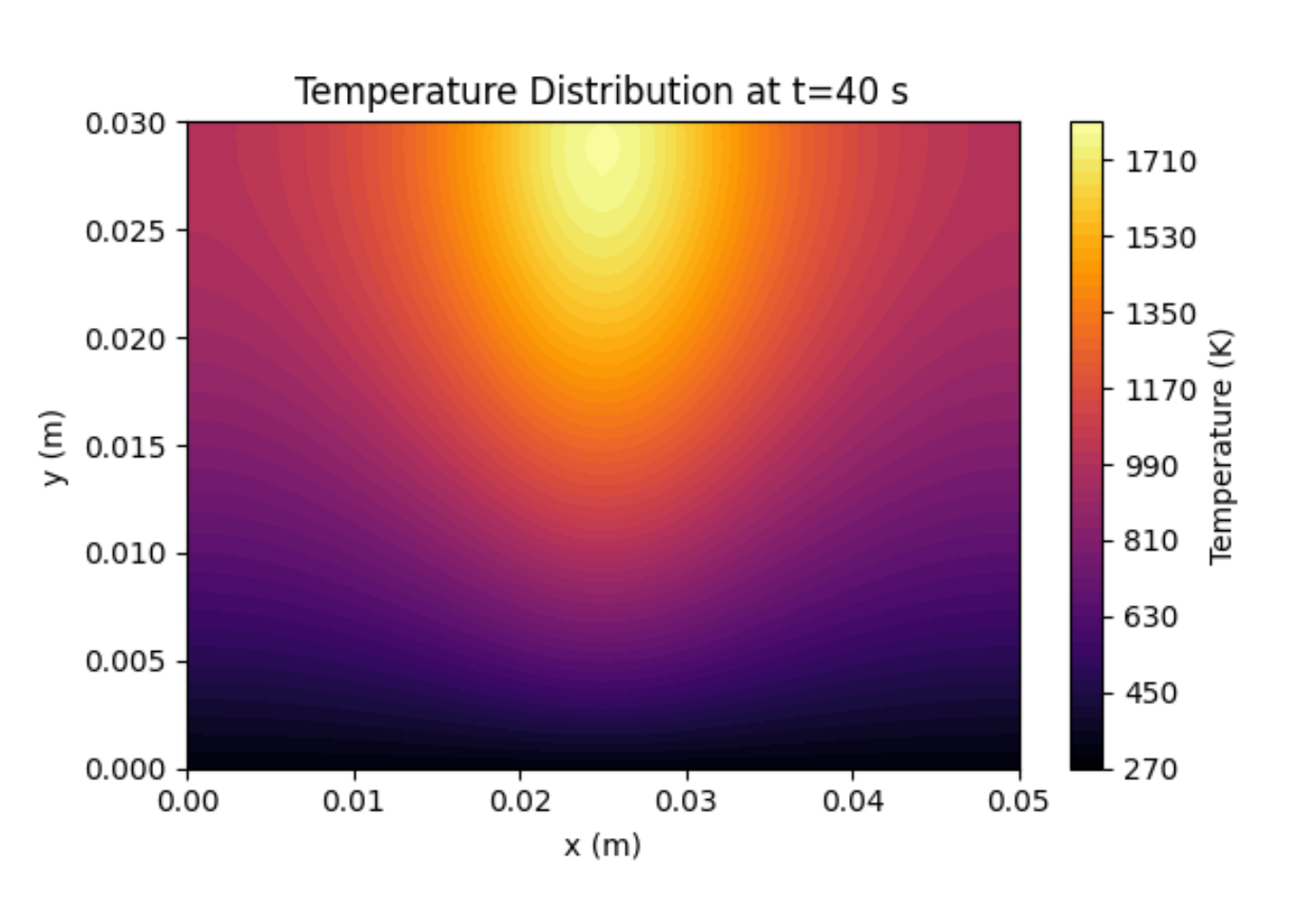
For the stationary-laser case, the volumetric source is modeled as
\[ Q(x,y,t) = \left(\frac{P}{w^2\sqrt{2\pi}}\right) \exp\left(-\frac{(x-x_L)^2}{2w^2}\right)f(y), \]
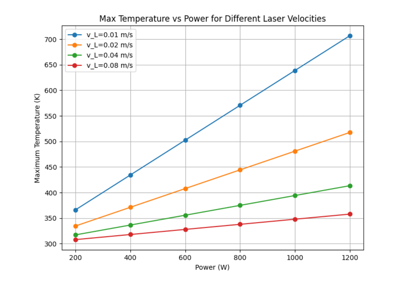
where \(x_L\) is fixed and \(f(y)\) describes depth attenuation. For a traversing laser,
\[ x_L(t) = x_{L,0} + v_L t, \]
so the source center moves in time while the update scheme remains unchanged.

This formulation preserves the dominant physics of surface heating, radiation loss, and moving-source behavior while remaining computationally efficient.

The explicit 2D heat solver was validated with a von Neumann stability analysis, which gave the condition
\begin{align}
\Delta t \le \frac{\rho c}{2k}\left(\frac{1}{\Delta x^2}+\frac{1}{\Delta y^2}\right)^{-1},
\end{align}
or equivalently
\begin{align}
r_x + r_y < 0.5.
\end{align}
Using
\begin{align}
\rho &= 7900\ \text{kg/m}^3, \\
c &= 470\ \text{J/(kg\cdot K)}, \\
k &= 48\ \text{W/(m\cdot K)}, \\
\Delta x &= \Delta y = 0.001\ \text{m},
\end{align}
the maximum stable time step was
\begin{align}
\Delta t_{\max} \approx 0.01934\ \text{s}.
\end{align}
Since the implemented value
\begin{align}
\Delta t = 0.01\ \text{s}
\end{align}
lies below this limit, the numerical scheme is stable for the chosen grid and material parameters.

Python was used to implement the full finite-difference workflow, including interior-node updates, nonlinear radiative boundary solves, stationary-source heating, traversing-laser heating, and post-processing for line plots, contour fields, and parameter sweeps. The resulting visualizations show depth-dependent temperature histories, final-time through-thickness temperature profiles, transient contour maps, and maximum-temperature trends versus power for multiple laser speeds.

The finite-difference simulation captures the dominant thermal response under localized laser heating with nonlinear radiative losses. For the stationary-source case, the maximum top-surface temperature increased from
\begin{align}
1661.53~\mathrm{K} \quad \text{at} \quad 30~\mathrm{s}
\end{align}
to
\begin{align}
1946.39~\mathrm{K} \quad \text{at} \quad 150~\mathrm{s},
\end{align}
showing rapid early heating followed by a gradual approach toward a limiting temperature as conduction and radiation balance continued energy input.

The solution predicts three key trends. First, temperature is strongly depth-dependent: the highest values occur at the heated top surface, while deeper regions remain cooler and respond more gradually. Second, the temperature field stays localized around the source. In the stationary case, contours show a concentrated hot region near the heating location; in the traversing case, this hot zone moves across the domain with the laser path. Third, the explicit scheme remained stable, since the chosen time step
\begin{align}
\Delta t = 0.01~\mathrm{s}
\end{align}
was below the von Neumann limit
\begin{align}
\Delta t_{\max} \approx 0.01934~\mathrm{s}.
\end{align}

Parametric results showed that laser power and traversal speed dominate the response. Increasing power raises the maximum temperature, while decreasing speed increases local heating by allowing longer energy deposition at a given location. Overall, the model reproduces the expected thermal behavior of laser-driven heating and provides an efficient framework for studying how source motion, power, and boundary radiation shape the temperature field.