FPGA Data Acquisition Platform

I am building this FPGA-based data-acquisition and instrumentation platform for mechanics experiments. It connects physical measurements to analysis: acquiring sensor data, timestamping each recognized data-ready event, checking the stream for missing or corrupted records, and converting raw counts into calibrated acceleration.

The current implementation pairs an Arty A7 FPGA with a three-axis Pmod ACL2 accelerometer and Python host software. As the instrumentation part of Project Hephaestus, its goal is to provide a dependable measurement foundation for vibration experiments and, later, additional sensing channels.
Status
Working accelerometer acquisition and accepted six-position calibration; development ongoing
Hardware
Digilent Arty A7 · Pmod ACL2 / ADXL362
Tools
SystemVerilog, Vivado, SPI, UART, Python
Focus
Hardware timing, data integrity, calibration, and signal analysis

Digital Accelerometer Test

Digital accelerometer tap test on a cantilever, with live acceleration, FFT, and wavelet views.

FPGA Acquisition

The acquisition chain separates sensor timing from computer-side processing. Rather than repeatedly reading the sensor on an unrelated polling schedule, the FPGA responds to its DATA_READY signal and timestamps the recognized event using a 100 MHz clock.

  1. Sensor → FPGA. A synchronized DATA_READY event triggers an SPI read of the X, Y, and Z channels.
  2. Acquisition → buffer. A FIFO queues sample records while the output link is busy.
  3. Buffer → computer. A packetizer sends framed binary records over the board’s USB–UART connection.
  4. Computer → analysis. Python validates the stream, saves raw binary and decoded CSV files, and produces time histories and spectra.

Each 17-byte packet carries a synchronization word, version, channel mask, timestamp, sequence number, three signed acceleration readings, and a checksum. The sensor determines the sampling cadence; the FPGA timestamps make that cadence measurable.

Data Integrity and Timing

The calibration campaign produced 86,389 complete packets across seven captures, with zero detected packet/header/checksum errors, zero sequence discontinuities, and zero binary-to-CSV mismatches. Timestamps remained monotonic after counter-wrap handling, and no samples reached the sensor’s digital limits.

The stationary capture measured 360.07 samples/s, compared with the configured nominal rate of 400 Hz. Rate variation across the six calibration inputs was 0.0344%. Analysis uses the measured timing rather than assuming that the nominal setting is the actual sampling rate.

Six-Position Calibration

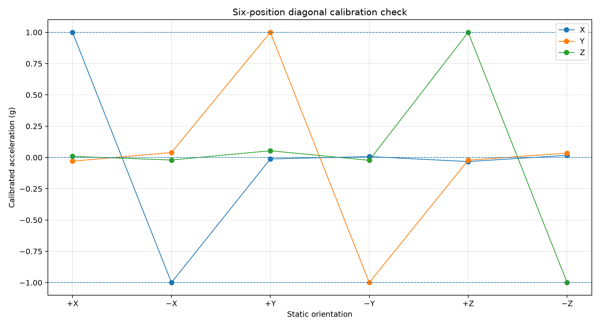
I used gravity as a reference by placing the assembly in six static orientations: +X, −X, +Y, −Y, +Z, and −Z upward. The paired positive and negative readings give an independent bias and sensitivity for each axis.

\[ \text{Acceleration in g}=\frac{\text{raw count}-\text{bias}}{\text{sensitivity}} \]

The resulting coefficients convert counts into g, or into m/s² by multiplying by 9.80665. This corrects per-axis offset and scale; it does not fit cross-axis coupling or mounting tilt.

Calibrated X, Y, and Z acceleration across six static orientations: each dominant axis reaches positive or negative one g while the perpendicular axes remain near zero
Six-position calibration check. Each point is an orientation mean; connecting lines guide the eye between separate captures. Open the plot for full resolution.
Fitted coefficients for the calibrated sensor and mounting
AxisBias
(counts)
Sensitivity
(counts/g)
X12.281011.20
Y43.261056.16
Z103.901048.44

Across the six fitted orientations, the maximum acceleration-vector error was 0.0549 g, and the maximum deviation of its magnitude from 1 g was 0.00150 g. A separate +Z repeat differed from the original calibrated mean vector by 0.00146 g.

Stationary Baseline

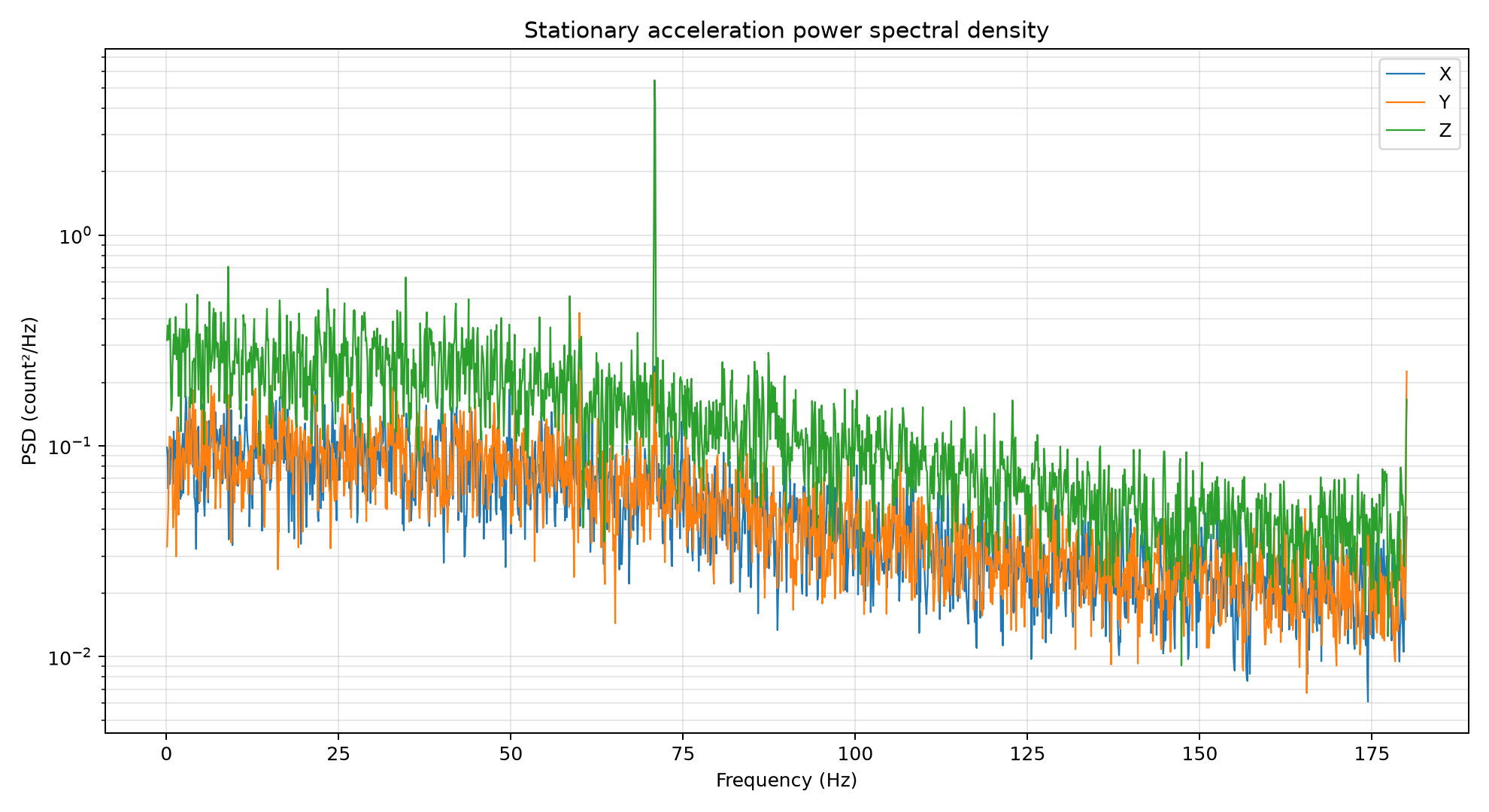
A stationary recording establishes what the assembled measurement system sees before an experiment begins. The retained baseline contained 20,521 samples over about 57 seconds, with calibrated sample standard deviations of 3.075 mg in X, 3.002 mg in Y, and 4.857 mg in Z, where mg means one thousandth of g.

Stationary X, Y, and Z acceleration power spectral densities in raw count squared per hertz, with a prominent Z-axis component near 71 hertz
Stationary power spectral density, shown in the original raw-count units. This is the as-mounted baseline, not a measured structural mode.

Follow-up stationary captures reproduced narrowband components around 58–60.5 Hz and 70–71.5 Hz without identifying a unique physical source. Future tap tests will use a session-specific stationary control and repeatable, tap-synchronous response to distinguish structural motion from the baseline.

Outcome and Next Steps

The platform now has a working path from sensor acquisition to timestamped, checked, and calibrated acceleration data. The current milestone combines a recorded packet campaign with no detected packet errors, accepted bias/scale calibration, and a repeatable stationary baseline.

The next stage is a repeatable cantilever mounting and tap-test workflow, followed by strain-gauge and analog acquisition development. Those extensions build on the measurement pipeline established here.