I built a breadboard computer using Ben Eater’s 6502 project as a starting point, then used it to run numerical methods in BASIC. Coming from mechanical engineering, simulating a physical system was one of the first things I wanted to try as I got into computer architecture.
Numerical Methods on a 6502 Processor
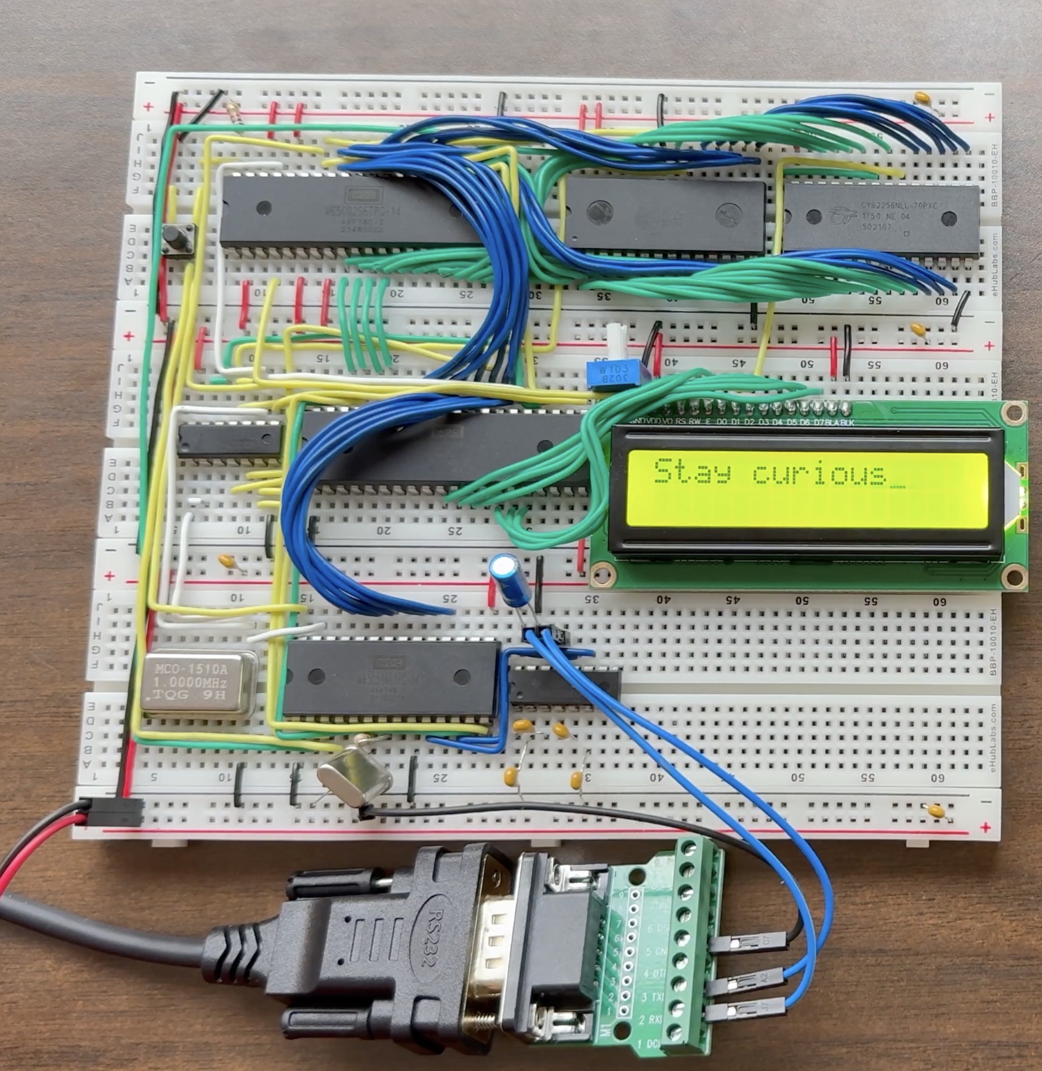
Runge–Kutta on a breadboard
I ran fourth-order Runge–Kutta (RK4) in BASIC to simulate the step response of a series RLC circuit. The program takes the circuit parameters and timestep through a serial terminal, plots the response with text characters, and reports the peak capacitor voltage, overshoot, and final state. The LCD shows when the calculation is running and when it is complete.
The underdamped example in the video uses R = 20 Ω, L = 100 mH, C = 100 μF, and a 5 V step. It advances in 0.4 ms steps over 200 ms of simulated time. The program reports a peak capacitor voltage of about 6.754 V at 10.4 ms, or 35.08% overshoot, before settling near 5 V.
| 6502 BASIC runtime | ~120 seconds |
|---|---|
| Python runtime | ~0.005 seconds |
| Reported 6502 RK4 error | 0.000184% |
Python was roughly 24,000× faster in this comparison. These figures describe the two implementations and setups, not the processors in isolation. The appeal for me was getting a numerical simulation to run on a computer I had wired together.
UART from first principles
I also studied UART communication to connect the breadboard computer to a terminal. This demonstration shows “Stay curious.” appearing in the terminal and on the LCD, with the terminal connection configured at 19,200 baud. That serial interface also lets the numerical program accept inputs and display more output than fits on the LCD.